Managing risk successfully at any level requires an understanding of a concept called “probability.” As both an insurance company (risk transfer) and a cyber risk management company, Resilience relies on understanding probabilities to price our services and to guide our clients to greater levels of cyber resilience. As we often receive questions from our clients about how Resilience develops the probabilities that inform the LEC (Loss Exceedance Curve) in their Edge Platform report, we’ve put together this accessible overview.
What is probability?
Before we can explain how we develop probabilities that support the risk analyses that inform our Edge Platform report, it’s important to clarify what we mean by “probability.” Though the term is often used in mathematical calculations, its meaning is more nuanced than it might seem at first.
Two schools of thought on probability
Old School
In our first exposure to probability in math classes, we learned that probability represents the average proportion or frequency of a particular event occurring relative to all possible opportunities for it to happen. For example, if we toss a coin a large number of times and record the number of times heads appeared (the event of concern), then divide the number of heads by the total number of tosses (opportunities for heads), the proportion could be taken as the probability of getting heads when you toss that coin. With some hand waving about the similarity to other coins, we could say that the probability of tossing any coin and getting heads is the same as our coin.
This idea presents a number of problems. We’ll consider three of them. First, the truly technical definition of probability requires a very large number of samples to establish a probability–an infinite number, in fact. Second, the system that generates the events for which we want to measure the probability needs to remain very stable. Finally, to accurately apply probability to individual cases and predict behavior, the individual must be almost identical to the reference population used to define the probability.
For example, if a person has certain known physiological characteristics and is exposed to certain environmental conditions, we might ask what the probability is that they will develop a particular disease, based on their similarity to a reference population. Fortunately, statisticians and actuaries have developed tools to address the challenges posed by these requirements, enabling informed decision-making even in cases that closely approach, but don’t fully meet, the ideal conditions. Unfortunately, they don’t work for a large number of situations in which we still need to make informed decisions and allocate valuable resources at risk. Cyber security is one such domain.
Old New School
While property and casualty insurers have a large volume and transparency of data relating security risk surface to loss claims, we often do not have the same quantity and quality of data in cybersecurity. Cybersecurity is also less stable compared to the systems typically covered by traditional forms of insurance. In our case, the source of threats and perils is driven by malicious intent. Threat actors learn and evolve in more sophisticated ways to accomplish their goals, making this domain much more dynamic and prone to instability than traditionally insured systems.
Finally, no two security configurations are the same. Each configuration has context-specific variations and exceptions, making it difficult to claim that two companies with similar security setups would face the same probability of losses. This is due to differences in organizational factors, environmental conditions, and prior technical debts embedded within their architectures.
An alternate school of thought about probability – that allows us to accommodate these difficult conditions, while still making use of the effective concept of probability – does exist. This approach was actually developed before the “probability is frequency” approach, but it fell into disuse for nearly a century due to the overbearing influence of a few significant statisticians. This school of thought, known as Bayesian reasoning (after the Rev. Thomas Bayes, 1702 – 1761), has resurfaced within the last few decades as a growing number of statisticians and scientists have recognized its power.
Simply put, Bayesian thinking views probability as a “degree of belief” that an event will occur, rather than as the long-run frequency of repeated trials. This approach acknowledges that an assessor’s difficult-to-quantify background knowledge and judgments should influence the probability assessment, while still incorporating support from any available quantified data.
Given the iterative way in which Bayesian reasoning is designed to update probabilities, it becomes a much more dynamic and flexible system for learning about one’s environment rather quickly, even when the environment is also changing quickly. Such a flexible system that can operate effectively on much smaller scales of data is exactly what we need in the domain of managing and transferring risk in today’s cybersecurity environment.
Does it work?
Considering this seemingly subjective way of thinking about probability, we might wonder how we can do anything valuable with it, such as managing risky assets or providing guidance about where to allocate resources to improve an organization’s cybersecurity. The answer has two parts.
First, although the notion of Bayesian probability seems subject to influence from individual perspectives and experiences, people who study and analyze risky things have developed an objective set of precise rules about how to use probability in calculations about those risky things. As long as the objective rules are followed consistently, we can draw informative inferences that support making valuable decisions, even when we have very little data. A long history of empirical evidence supports this claim.
This brings us to the second part. It’s not just that we’re luckier when we use probabilities with these precise rules. Risk managers have also learned that when you try to use approaches for analyzing risks that are not consistent with the precise rules of probability (like using heat maps), really bad things can happen—like losing a lot of money or a lot of lives. You tend to be less lucky to a higher, more impactful degree.
At Resilience, we understand this deeply, which is why we work hard to ensure our cyber risk models are both accurate and logically consistent. This not only provides you with valuable guidance but also helps us manage our own risk portfolio to achieve competitive returns.
Regardless of the subjective nature of many of the components of our model probabilities, our application of the rules of probability and our “skin in the game” provides the incentive to develop probabilities that earn confidence in their accuracy.
The structure of the Resilience risk models
Simple event trees
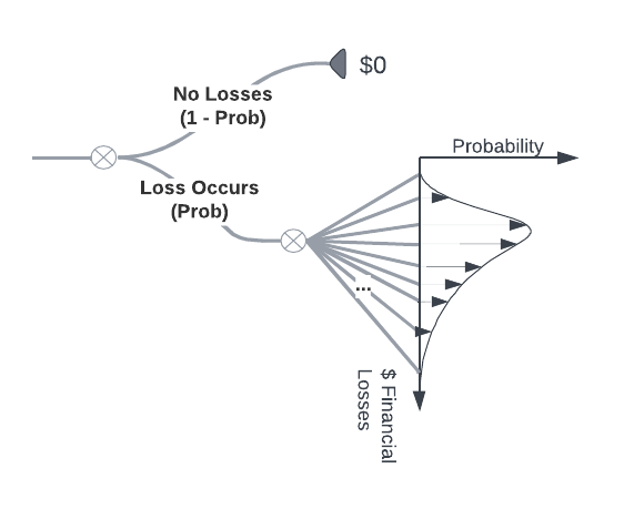
At the most basic level, the Resilience risk models take the following form of a simple event tree:
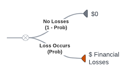
This tree represents the idea that over some period of time, either financial losses occur with a measured probability (Prob) or do not occur with a complementary (1-Prob) probability. We call this a discrete probability event. Since no one can exactly predict the loss values before they occur, we also represent losses with probabilities.
However, since losses can take on values across a continuous range, we use a probability distribution to represent them. It might look something like this:
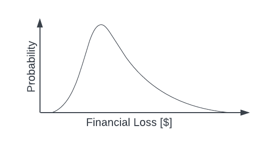
We can think of the probability distribution as an event “bush.” Instead of a small number of clearly delineated branches in an event tree, the event bush has many branches. The branches occur at each point along the Financial Loss axis and point to the Probability that any loss value occurs, indicated by the distance from the Financial Loss axis to the curve.
Signals and triggers
Of course, our models are not as simple as the toy illustration above. Our complex models are constructed as a network of event triggers and input signals that, when taken together, inform the probability that losses will occur, the range of losses when they do occur, and the probabilities associated with the size of the losses in the range. We do this according to the kind of perils that can materialize into those losses. The kinds of perils we consider are business disruption, data breach, fraud, and extortion. The real model looks similar to the following node diagram.

The rate at which perils result in losses is influenced by the maturity of the control measures reported by our customers. We tune the relationship between these signals, their level, and their output based on our internal subject matter experts’ degrees of belief, cyber claims data, and firmographic data. It’s a large network that facilitates the probabilistic reasoning described earlier. Given our understanding of applying the rules of subjective probability and our “skin in the game,” the results we observe are quite accurate.
The LEC
We bring all the probabilities together into a single graphical representation called a Loss Exceedance Curve (LEC). The LEC depicts both the probability that any loss events occur and the probability that any losses that do occur will exceed a given value.
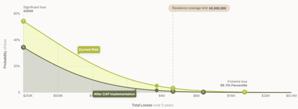
We can interpret the peak of the light green section of the curve, marked at 55%, as the probability of any loss occurring. This corresponds to the lower branch of the event tree shown earlier.
The rest of the curve is related to the event bush that we call a probability distribution, but it is a variation that cumulatively sums all the probabilities “backward” from right to left. Instead of telling us the probability that a precise loss value will occur in a given time frame, it tells us the probability that losses will be greater than a given value in the time frame. Assuming this curve (the light green portion) represents the risk profile of an organization over the coming three year period, we can read it in the following way:
- Over the next three years, we believe (given all the evidence we have at hand) there is a 45% probability that we will not experience any material financial losses ($0) and a 55% probability that we will experience material financial losses greater than $250K.
- There is a 20% probability that we will experience losses in excess of $1M and a 10% probability that our losses will exceed $2M.
- There is a 2% probability that losses will exceed the coverage limit of $5M.
The light green curve might indicate the risk profile of an organization that has very basic controls in place. The lower gray curve might indicate that same organization if they were to implement more advanced and significant controls. The effect would be that the probability of no material losses increases to 65%, while the probability that any material losses occur reduces to 35%. The probability that material losses would exceed $1M reduces to 10%; 4% at $2M. Exceeding the coverage limit falls to 0.5%.
Summary
Contrary to popular usage, probabilities are not simply the proportion of the occurrence of one event relative to the number of all possibilities of the event. They represent a much deeper idea related to the background information about conditional influences and causal relationships to events that are difficult to formalize completely.
Of course, this background information should include the observed proportions related to the event, if possible to obtain them. However, the real purpose of probabilities is not to satisfy esoteric mathematical definitions but to support our ability to make important decisions under uncertainty.
So although probabilities are based on subjective information, when used in an objective framework, they demonstrate an effective way to improve the value of those risky decisions we make.

