This blog post is a supplement to the webinar Richard Seiersen and Robert Brown delivered on April 5, 2023.
In our first webinar, Building the Defensible Security Budget, we introduced the idea of using influence diagrams to visually capture the essence of the security events we want to control with a strategic budget and their combined effects in financial terms, such as Treasury Risk (observed in Realized Losses) and Return on Controls. This thinking tool helps you build the narrative that speaks to the concerns of the “Money People,” such as CFOs. Learn more about making them your allies here.
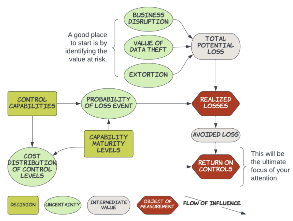
Influence diagrams are a powerful way to represent the qualitative essence of the structural relationship between events and outcomes, whether those events are decisions we make or events outside our control (uncertainties). Our first influence diagram represented one that contains security control decisions that conditionally affect the probability that a ransomware loss event can occur. For our discussion here, we remove the effect of those decisions so that we can focus on Value at Risk (i.e., Realized Losses) before we spend money to control it. That way, we can get an idea about how to prioritize our attention on the security perils that matter most. Now, the probability of a loss event will just be the base rate probability that any material ransomware event occurs regardless of controls in place. For illustration purposes, we set this base rate probability to 2.5% per year.
The top three green uncertainty nodes (i.e., business disruption, the value of data theft, and extortion) represent placeholders for the costs that could be incurred when a loss event occurs. These will need to be accounted for as actual numerical values in the financial model that you build to support a defensible budget.
You might think that developing a value for those would be as difficult as lifting an elephant. Yes, that could be difficult, but not impossible, particularly if we know approximately how much elephant we need to lift. So, before we attempt to lift an elephant, it would help us to develop an estimate of how much an elephant weighs if we don’t have that information readily at hand. Let’s try that here.
Of course, we might be concerned about what kind of elephant we are referring to since elephants come in a range of sizes, depending on whether we’re thinking about African elephants or Indian elephants, males, females, or adolescents. So the first thing we should specify is exactly what we mean by “an elephant.” We will define an elephant as an adult male African elephant. That helps us to narrow our space of consideration and reduce the ambiguity about what kind of elephant we mean, but it still leaves open a range of possible weights. This implies that our estimate will have to be stated as a range.
This may still feel like a daunting task to us. After all, we’ve only seen a real elephant at the zoo once or twice, and the other times we’ve seen one on National Geographic, either on television or in the magazine. It’s difficult for us to have a close-at-hand experience that we draw on to estimate directly. So maybe we could think about elephants in terms of something a little more familiar, like adult dairy cows. Most of us are probably a little more familiar with the size of a cow. But if we aren’t, we might consult the subject matter expertise of a cowboy or rancher.
But even with this further decomposition, we might still feel too removed from the daily cow experience to provide a good judgment. So let’s decompose an adult dairy cow into terms of an adult US male. The point is that we are thinking of the problem in objects and units that are familiar to us. Once we understand that familiar level, we can integrate back into the whole unfamiliar elephant.
As an approximation, let’s use 200 pounds as the average weight of an adult US male. Maybe we think of 3 to 7-unit adult males fitting into an adult dairy cow. Simple arithmetic tells us that the range of weight of an adult dairy cow might fall between 600 to 1400 pounds. Now we take a simple average of that to get 1000 pounds. Repeating that process, we estimate somewhere between 4 to 11 adult dairy cows could fit into an adult African male elephant. Using the 1000-pound average weight for the cow, we now update our belief that the weight of an adult African male elephant falls between 4000 to 11,000 pounds.
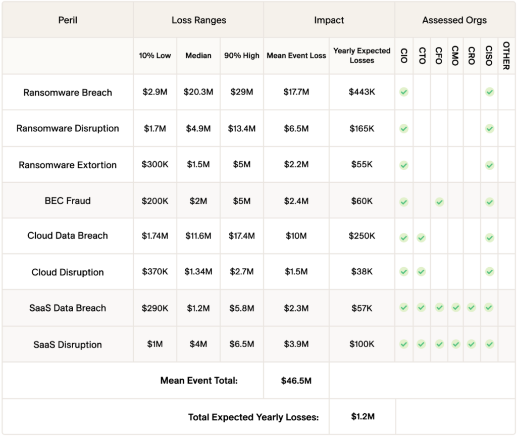
Up to this point, we have assumed that information about elephants is not readily available. Now let’s say we have access to some historical information provided through resources like Google or Wikipedia. Consulting those resources tells us that the range of weight for an African adult male elephant falls between 4000 and 14,000 pounds. That overlap is not bad. It tells us that we are calibrated both for accuracy and precision. Of course, that might not always be the case, but our simple example demonstrates that we can sometimes effectively produce reasonably good estimates about unfamiliar things by decomposing them into familiar unit reference objects. Eventually, we will replicate this process when we apply it to the Value at Risk we face through cybersecurity perils, as we might tabulate in the following table (please note that the values in the table are for illustrative purposes only).
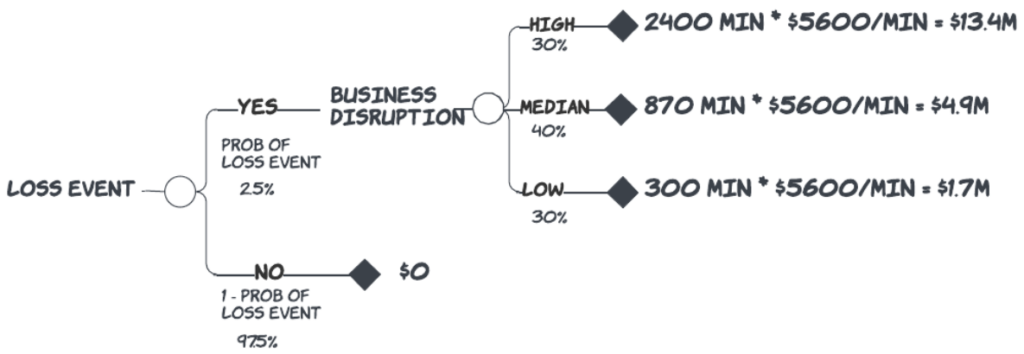
Let’s return to our ransomware value at risk exercise. We want to convert our qualitative influence diagram into a computable form called a decision tree or an event tree. The first step in this process is to identify the initiating event. For our case, this would be the Loss Event because we won’t incur any ransomware losses unless a material, reportable event occurs. For this event and all other events, we will need to identify three specific kinds of information: the event possibilities, their probabilities, and their end values.
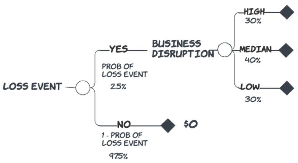
Now, we assign probabilities to the branches, which are the possibilities. On the Yes loss event, we will use the probability, as we’ve already stated, of 2.5% per year. The No loss event will be one minus that value, or 97.5% per year. (It’s important to remember that the probabilities of all possibilities in an event must sum to one.) On the branch where we know the explicit end value, we go ahead and assign it. In the case of No loss event, the end value is $0.
On the Yes loss event branch, we assigned the possibilities for each of the sub-components of the potential loss. Since we treat them as occurring simultaneously in our simple example, we can show them as a cascade. For each one of the sub-components, we identify their possibilities as a high-value case, a median-value case, and a low-value case.

To simplify our efforts at this point, we can deal with the business disruption component apart from the data theft and extortion components. How we handle business disruption can simply be replicated for these other two.
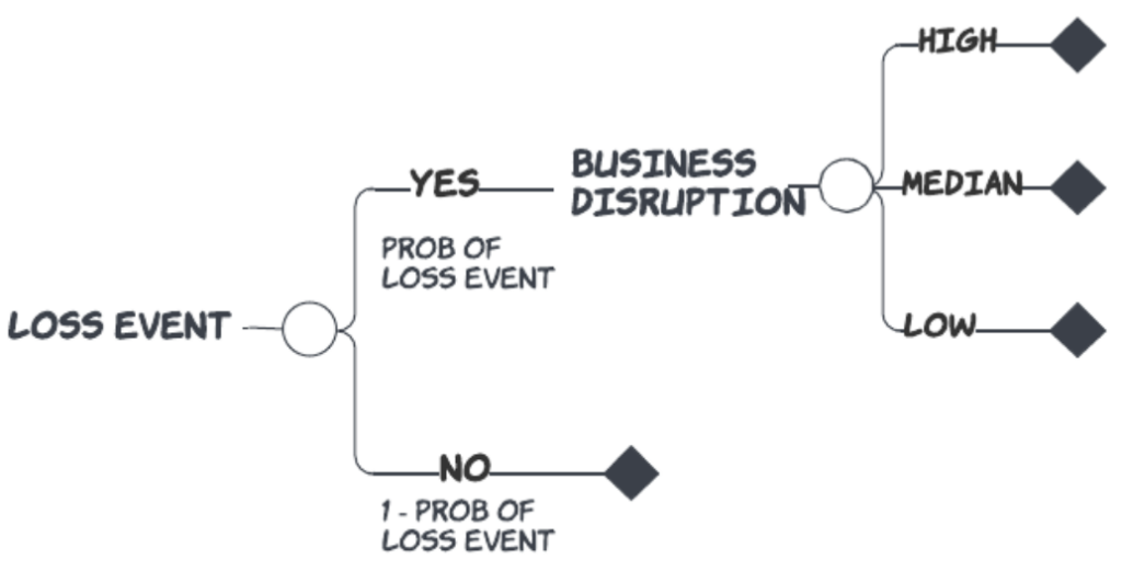
It will be helpful if we think of the high, median, and low cases as discrete points in an 80th percentile prediction interval, for which we think of the low case as a P10, the high case as a P90, and the median case as the P50. To clarify, we think of the low case as representing the outcome for which there is a 10% chance that the actual value could still be lower, and we think of the high case as the outcome for which there is a 10% chance the actual value could still be higher. Finally, we think of the median case as the outcome at which we are willing to bet coin toss odds (or 50% probability) that the actual outcome would be higher or lower than that value. Fortunately, we have a standard set of rule-of-thumb probabilities we can use for these P10-P50-P90 values, namely, 30%, 40%, and 30%, respectively.
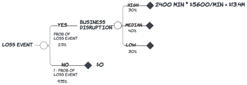
Now we can think of the values to assign to the possibilities. Let’s start with the high case first to nudge us out of the wishful thinking that the outcome might not be as bad as we anticipate. After thinking about our security configuration, we anticipate in this almost-worst case, we could restore business operations in 2400 minutes from the start of a disruption.
We’ve also given some thought to how much business disruption costs on a per-minute basis. This cost of business disruption could be based on deferred revenue, unrealized productivity from essential resources, increased inventory carrying costs (for much longer disruptions), etc. Of course, this number could also be represented as another range represented as a set of possibilities and probabilities, and it would most definitely be different for every business. However, here we are using $5600 per minute as a proxy in our simplified discussion. You could think of this as the unit adult male that we are now fitting into our representative cow. The value for this high value would be $13.4 million.
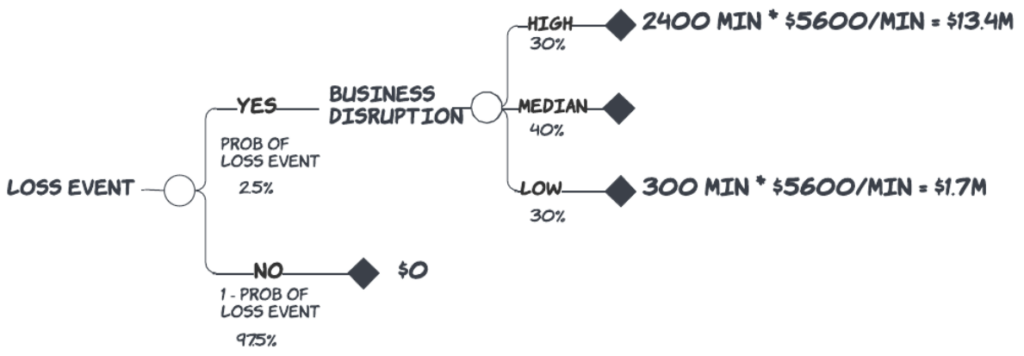
Next, we think about the low case. We assign 300 minutes of disruption to our almost best-case condition. The cost for this case would be $1.7 million.
Finally, we assign 870 minutes to our median case disruption for a cost of $4.9 million.
The value of thinking in this order—high, then low, then median—helps us avoid a few common thinking pitfalls, one of which I’ve already mentioned – wishful thinking. By thinking about the outside edges first and the centerpoint last, we also avoid anchoring on our first available impression and then adjusting for a range with an ad hoc variance like +/-20%. We are effectively controlling for cognitive bias and commitment to an unjustified level of precision before it is warranted.
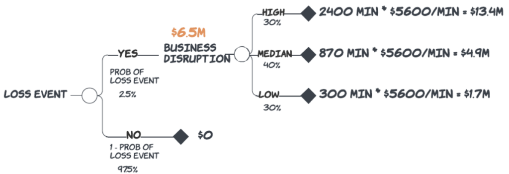
Now that we have values for the possibilities of our business disruption event, we can calculate our unit cost for business disruption by multiplying the value of each possibility by their respective probabilities. We call this unit cost the Mean Event Loss for business disruption.
Mean Event Loss = (0.3 * $13.4M) + (0.4 * $4.9M) + (0.3 * $1.7M) = $6.5M/yr
We perform the same rollback calculation with the loss event to get the Expected Value of Realized Loss for business disruption.
Expected Value of Realized Loss = (0.025 * $6.5M) + (0.975 * $0) = $163K/yr
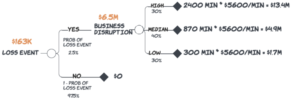
By “expected value,” we don’t mean that this is a value that you should anticipate to actually materialize and show up as a cost on your P&L or balance sheet. It’s a statistical term that refers to the probability-weighted value of all possibilities that you face in a given event. In some cases, expected values cannot even occur, but they still provide us with a consistent means to compare different events with different ranges of possibilities (but the same units) and probabilities. If we repeat this Value at Risk process for the remaining ransomware components, as well as other cybersecurity perils, we will have a mathematically rigorous and logically consistent way to prioritize our attention on the most impactful perils first to develop our control strategy.
I mention here a caveat. We should be careful not to think only in averages, which we refer to as the “flaw of averages.” If one of the high values for a peril exceeds approximately 15% of your total asset value, you will need to give it more attention than the simple expected value would imply. In other words, the tail could exceed your company’s risk tolerance, and due diligence would require a more rigorous treatment of the event for which that tail is associated.
If you missed our first webinar in the series, you could read our blogs on How to Make the CFO your best advocate (part 1 here, part two here).
We’d love to know if you enjoyed this article or have different thoughts about what we discussed here. Please, let us hear from you! It makes all the effort put into these articles much more worthwhile.
Finally, we will also be running full training sessions in San Francisco during the RSA conference and in Atlanta during the RIMS conference. Registration links for those sessions are listed on our Events page.

